Uncertainty Studies and Modelling

Overview

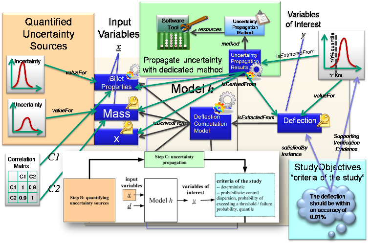
Uncertainty modelling wraps around a simulation as shown below.

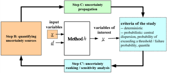
Simple method ‘h’ with inputs ‘x’ and outputs ‘y’

Here simple method h has inputs z and outputs y. The quantified uncertainties for the inputs are determined (orange), and the propagation to the Uncertainty on the output is computed (green), based on the analysis requested by the Study (cyan).

Single step intermediate computation example

This section builds up the overview picture using a scenario from the Very Simple Example. The first step is to determine the input-method-output objects. This is shown below:

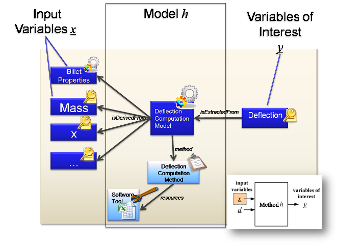
Simple Deflection Computation Method ‘h’ with Billet properties, mass, etc ‘x’ and outputs Deflection Computation Model ‘y’ The Uncertainty values for the inputs are then determined. These are shown as parametric distributions in the example because they are based on manufacturing processes with inherent variability. The example also shows a Correlation matrix between two of the inputs. The values here are low, meaning that there is very little Correlation between the material properties and the mass.

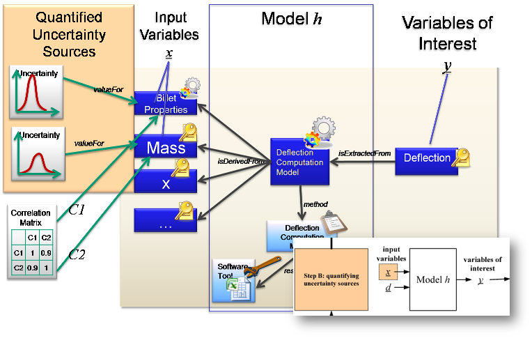
Uncertainty and Correlation on the inputs

The Requirement that the Uncertainty of the output must be within a certain quartile is added to the output. This means that the uncertainty objects are anticipated on the outputs, but without the values yet computed. Effectively the Deflection will satisfy the requirements, and the uncertainty value will be the evidence for the verification. (see also Requirements and Verification)

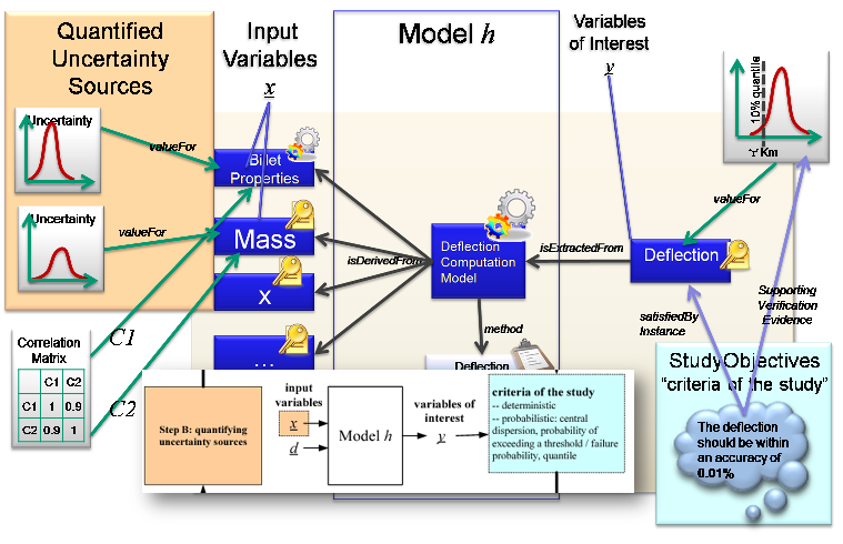
Requirements for the output to have a particular uncertainty

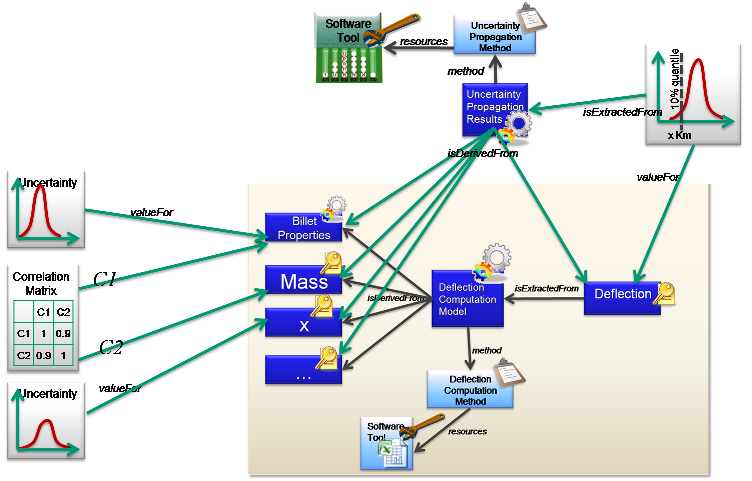
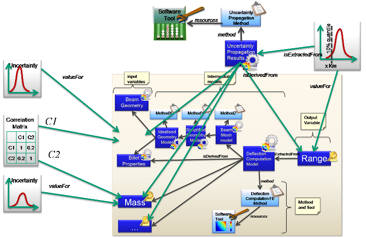
Finally the method to compute the propagation of the Uncertainty from the inputs to the outputs is added (in green). This is a new model to compute the uncertainty that has the same inputs as the deflection model, but this method will use the uncertainties and correlations associated to them. It has a method and tool associated to show how the uncertainty model was computed. Finally the uncertainty value is extracted from the model. This provides the full traceability of what is planned, and after the computation, what actually happened.

Uncertainty Propagation Results model added, with method and tool. Provides traceability for uncertainty values.

So far this example has assumed that the output Uncertainty can be computed from the input uncertainties as shown below. (Note: The “Uncertainty Propagation Results” node may not actually have any “results” attached at the end of the analysis, but it is needed as a place to capture the who/how/when/etc meta-data for the quartile computation).

Computation of output uncertainty from input uncertainty values

In the case where the “Uncertainty Propagation Method” uses sampling techniques, the input uncertainties and Correlation information are used to set up several “runs”. The results from these runs are used to compute the Uncertainty on the output(s). The “final” output is given a value above the required uncertainty quartile.

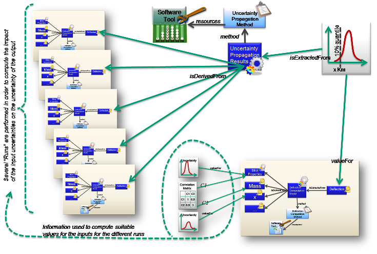
Computation of output uncertainty from sampling iteration runs.

There is no limit to how complex the “Model h” can be. The example below shows that it is actually an associative network of models that are to be computed to get from the input uncertainties to the output uncertainties.

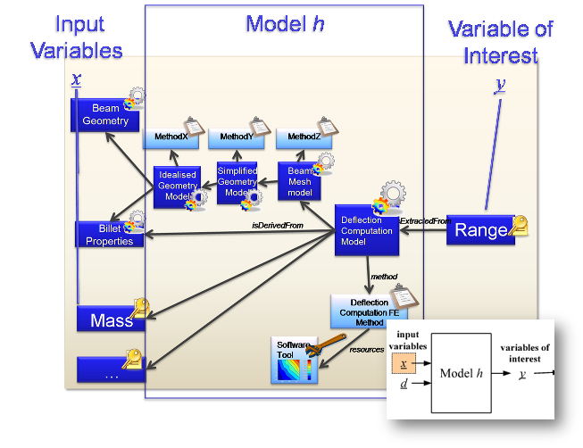
Associative Model Network used to compute “Model h”

As with the simple example above, the uncertainties, and propagation methods are added as shown below:

Uncertainty on inputs and outputs for the Associative Model Network

Worked example using Business Object Model Classes

In the example, a first study is carried out to compute a deflection. This proves satisfactory, but with insufficient accuracy. A second study is carried out, with the same requirement for maximum deflection, but with an additional objective for greater accuracy. During the work of this study it was found that the results are very dependent on the material properties, and so a new requirement is added to constrain the variability of the material properties. This new requirement has its source as the second study, and is traced to the objective for that study.

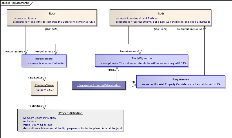
Study objectives as requirements

The elements of the two Associative model networks for this scenario are shown below.

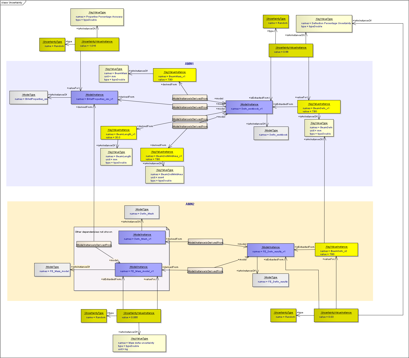
Two AMNs with uncertainty values

The final traceability relationships show that it is the BeamShellSolid ModelInstances that must satisfy the requirement for deflection, and the evidence used to verify satisfaction of this requirement are the BeamDeflection KeyValueInstances. Similarly the accuracy requirement must be satisfied by the BeamDeflection KeyValueInstance, and the verification evidence is to be provided by the deflection analysis results and the Uncertainty value that is extracted from them. This is illustrated below.

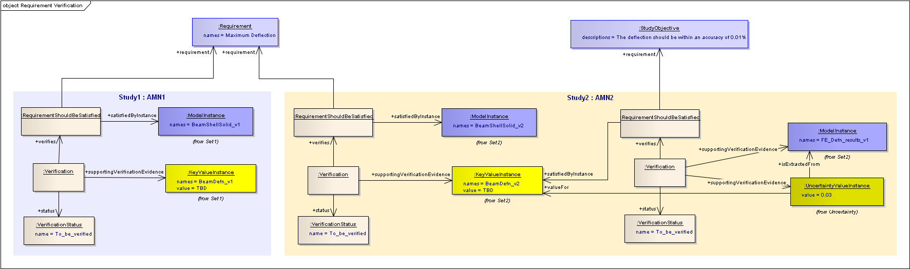
Requirement Verification

For more details and the background on this example, see: Introduction to the Very Simple Example.

Optimisation and Uncertainty

Optimisation Equivalent

The diagram below shows the set-up for an Optimisation of an Associative Model Network. The inputs have a range associated with then. This is modelled as a continuous uniform distribution. This is the same distribution class that is used to describe the normal distribution for an Uncertainty on the input.

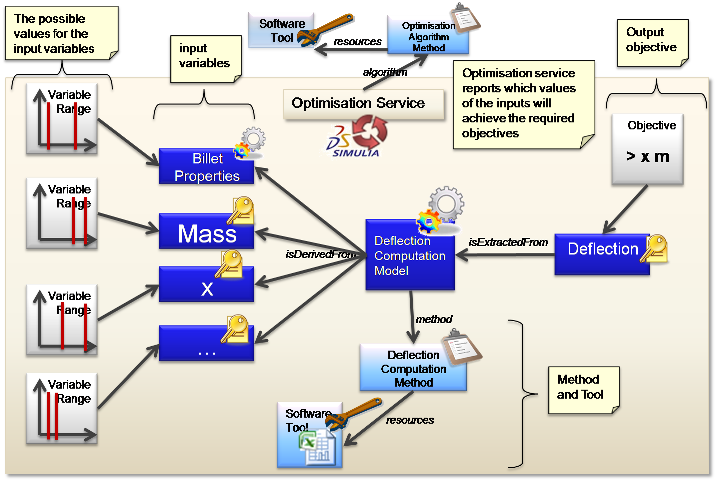
Optimisation of an Associative Model Network (without uncertainty)

Correlation allows you to reduce the number of iterations, as some combinations of input variables will not occur.

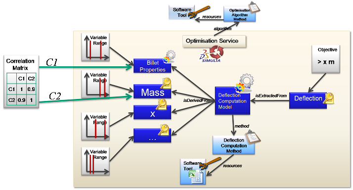
Optimisation with correlation between the inputs.

Several “Runs” are performed in order to compute the values of the inputs that will achieve the objective(s). The runs can be series or parallel depending on the type of Optimisation. If the optimisation is a “design of experiments” there may be an additional run at the end to prove the conclusion. For an iterative optimisation, the final run will be the result.

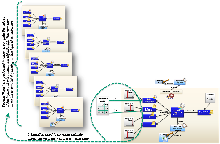
Optimisation runs with correlation between the inputs.

Optimisation and Uncertainty parallels

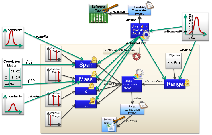
As can be seen from the above examples there are many parallels between an Uncertainty Study and an Optimisation Study. These are illustrated below.

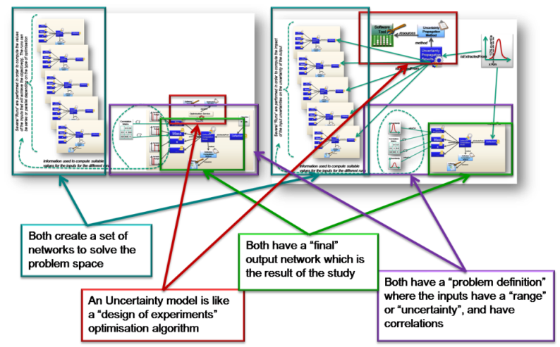
Illustration of the parallels between an optimisation study and an uncertainty studt

Combined Optimisation and Uncertainty

The diagram below shows a combination of Uncertainty on the input variables, which have some correlations defined. All feeding into an optimisation with the results analysed and an uncertainty on the outputs computed.

Combined Uncertainty and Optimisation with correlation.

Enterprise Architect Documentation

See SysML - Uncertainty for more details.

Section author: Judith Crockford